Traffic Sign Classification
German Traffic Sign classification using deep learning.
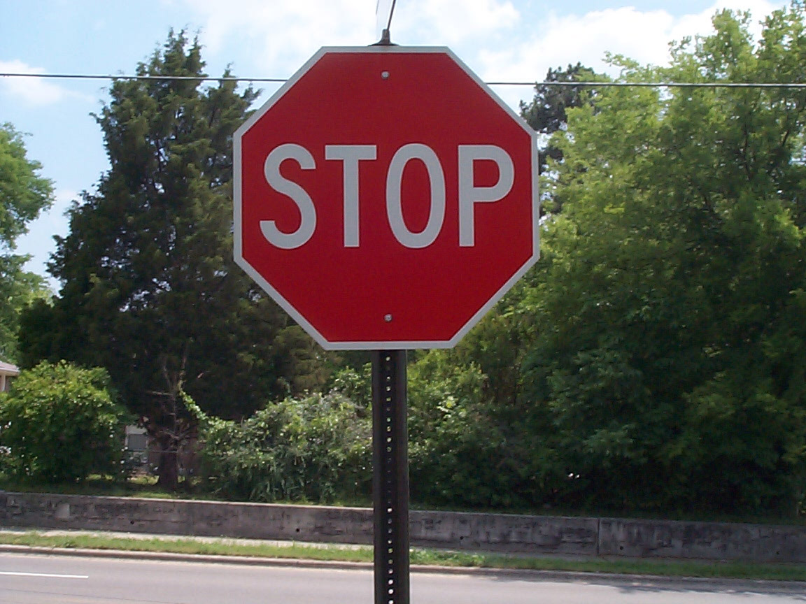
 Image credit: Google Images
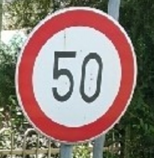
Goal : Build a Traffic Sign Recognition Project
The goals / steps of this project are the following:
- Load the data set.
- Explore, summarize and visualize the data set.
- Design, train and test a model architecture.
- Use the model to make predictions on new images.
- Analyze the softmax probabilities of the new images.
The Data Set - A look inside
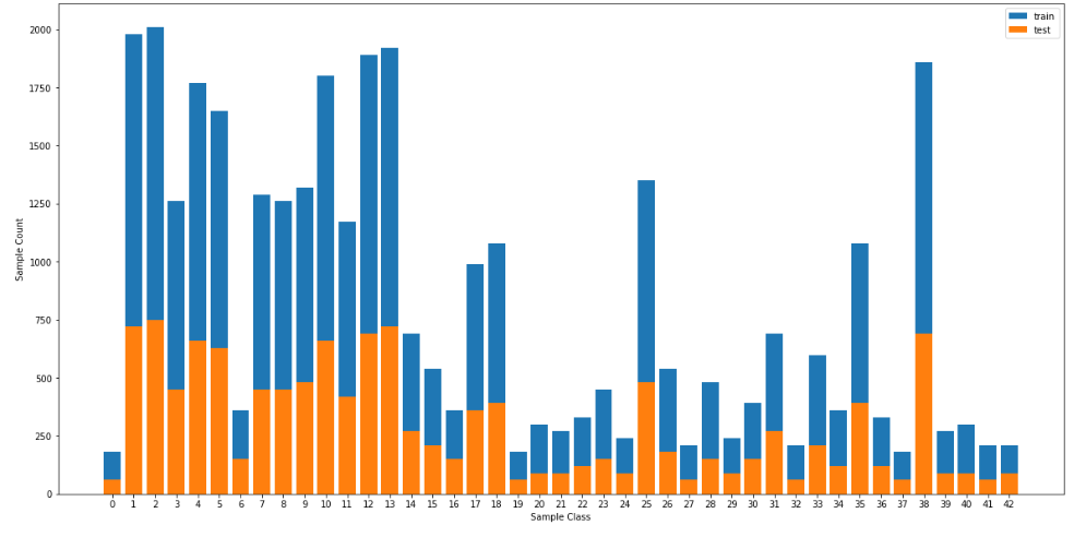
The dataset used for this project is German Traffic Sign Dataset which cabn be downloaded from here. Python's numpy library was sufficient to get the job of getting data statistics done here. Here's the summary:
- The training set consists of 34799 images.
- The testing set consists of 12630 images
- All the images are 3 channel, sized 32 by 32 pixels.
- There are a total of 43 unique classes in te dataset.
Here's a nice image for those souls who didn't bother reading that statistics stuff.
Pre-Processing
Now it's the time for the "pre-processing" of data. Nah! Let's skip it for now and see if it really matters of is it just another piece of jargon thrown around.
The Model
Well, let's start with something simple. The LeNet architecture is probably the first thing that comes to mind when we think of using a pre-existing architecture. So we will use that.
Basic LeNet Architecture
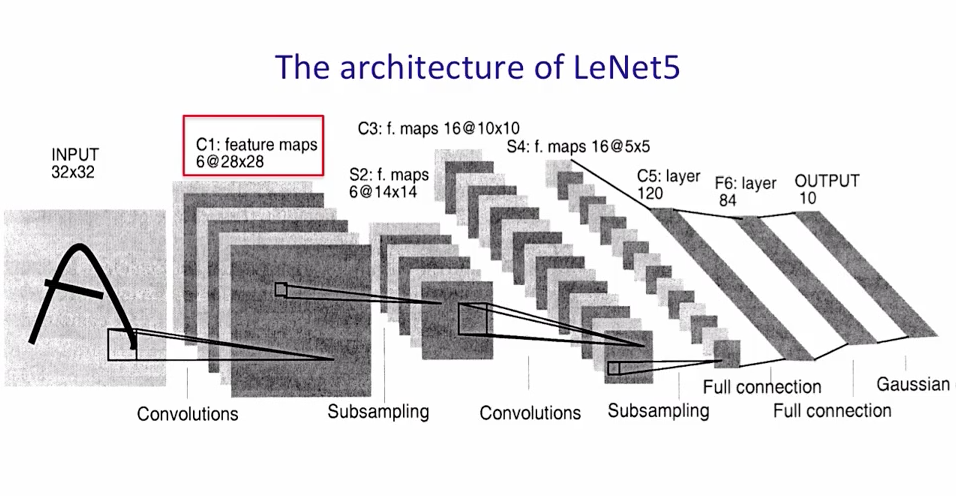
The Architecture looks like this:
My final model consisted of the following layers:
| Layer | Description | | --------------------- | --------------------------------------------- | | Input | 32x32x3 RGB image | | Convolution 5x5 | 1x1 stride, valid padding, outputs 28x28x6 | | RELU | N/A | | Max pooling | 2x2 stride, outputs 14x14x6 | | Convolution 5x5 | 1x1 stride, valid padding, outputs 10x10x16 | | RELU | N/A | | Max Pooling | 2x2 stride, outputs 5x5x16 | | Fully Connected | Input - 400 Output - 120 | | Fully Connected | Input - 120 Output - 84 | | Fully Connected | Input - 84 Output - 43 |
The Training
Now that the architecture is finalized, let's set the hyperparameters. Learning rate -> 0.0005. Let's play it safe the first time. If the training is slow, it could always be increased.
Epochs-> 60
Batch Size-> 32
Optimizer-> Adam Optimizer
Pull up your sleeves, folks. It's time to train. Pressing Cmd+K. Yea, now we can sit back.
The Result
| Accuracy Type | Accuracy Value | |:---------------------:|:---------------------------------------------:| | Training | 99.99% | | Testing | 91.085% | | Validation | 92.562 |
That's not bad for a start. 92.562% validation accuracy and 91.085% testing accuracy. And a whopping 99.99% training accuracy (Did I hear someone say overfitting?). And we didn't have to do anything for that. Everything out of the box. And it does seem pre-processing is just another fancy term after all.
So that's it ? Should we pack up and go home now ?
"What about dropout?"
"What about regularization?"
"What about other activation functions?"
"What about other architectures?"
"How about testing with some pre-processing and then coming to any conclusion?"
Okay, okay!! Let's try those points and show everyone once and for all why almost everything is overhyped these days
Digging deeper
Let's test on 9 additional images and see how our model performs.
The Report Card
Additional Data Accuracy -> 80%
| Actual label index | Predicted label index | Highest softmax probability value | 2nd highest softmax probability value |
|---|---|---|---|
| 18 | 18 | 1.00 | 0.00 |
| 1 | 1 | 1.00 | 0.00 |
| 14 | 25 | 1.00 | 0.00 |
| 34 | 34 | 1.00 | 0.00 |
| 2 | 2 | 1.00 | 0.00 |
Oh boy! Our model at the moment is acting like a arrogant and overconfident brat. It never has any doubt regarding what it thinks the right answer is. Even when the answer is wrong.
Time to don the detective hat
So, lets revisit the data and look closely at the class distribution for the classes involved in additional testing we performed.
| Class index | Number of images for this class | |:---------------------:|:---------------------------------------------:| | 1 | 1980 | | 2 | 2010 | | 3| 2010 | |13 | 1920 | |14 | 690 | |18 |1080 | | 23 | 450 | |25 | 1350 | | 26 | 540 | |28 | 480 |
Our model gets right the class labels 18, 1, 3. Our model gets right the classes for images which have large number of image samples, and gets wrong which don't have that many in the training data.
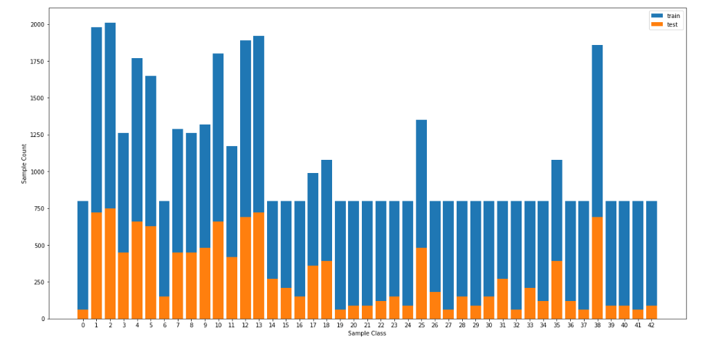
Lets sort this out. "But How?" Time to put to the concepts of oversampling and undersampling to use. Let's increase the number of images for classes having training samples less than a certain threshold.
Let's set the threshold to 800, i.e. let's increase the number of samples for each class having image samples less than this threshold to this number.
Now shall we test it out?
| Accuracy Type | Accuracy Value | |:---------------------:|:---------------------------------------------:| | Training | 99.8 % | | Testing | 91.801% | | Validation | 92.404% |
Some improvement is there.
On testing upon the additional data, the softmax probabilities came down from their pedestal of 1.00 to a range of 0.95. Which means there are doubts creeping in compared to before. But is it worth the hype ?
Let's go all the way and find out for ourselves.
Let's "Pre-process" the data for real. Let's:
- Convert the data into greyscale. (When it doesn't even matter, simplify, a.ka. Ockham's razor principle).
- Normalize the data. They say it helps in faster convergence.
- Further augment the data. Instead of replicating images, create modified versions of images with difference in brightness, translation, rotation etc The point is, give that spoiled, arrogant model a variety of data to learn from so that he doesn't cram his way through the examination.
- Do histogram equalization. (Even out the contrast of the image).
Here's the new data distribution:
| Accuracy Type | Accuracy Value | |:---------------------:|:---------------------------------------------:| | Training | 98.6 % | | Testing | 93.072% | | Validation | 93.651% |
Okay, so now we have jumped from 91.085% testing accuracy without pre-processing to 93.072% testing accuracy with pre-processing.
Lesson #1:
"I will never ever dismiss data pre-processing as a hype."
"I will never ever dismiss data pre-processing as a hype."
"I will never ever dismiss data pre-processing as a hype."
"I will never ..."
Dropout and Regularization
Now there's one more hype to be looked into. Overfitting. And how certain techniques like dropout and regularization can help prevent it. Let's see if it indeed is the case or not.
Let's first test dropout on the fully connected layers along with l2 regularization.
Woah!!. Testing accuracy of 95.044% . Some improvement that is. Let's go all the way. Lets apply dropout on all the layers.
Wait what ? 88.155% testing accuracy ? Training accuracy of 71.7 ? Why did it go down ? Oh wait. Maybe the reason is, the probability forkeeping nodes is 0.5 for all the layers, which would end up removing large number of nodes from the first few convolution layers which is resulting in underfitting. Let's set the that probability for convolution layers to a higher values and decrease the value with each subsequent layer.
| Accuracy Type | Accuracy Value | |:---------------------:|:---------------------------------------------:| | Training |82.4 % | | Testing | 95.532% | | Validation | 97.732% |
Yup. Now it's working fine and there's an improvement, albeit a slight one.
So the accuracy has jumped from 93.072% without any regularization (L2-Loss and dropout)to testing accuracy to 95.532% accuracy with both of these.
Lesson #2:
"I will never ever do the mistake of dropping out dropout layer from my convolutional neural network."
"I will never ever do the mistake of dropping out dropout layer from my convolutional neural network."
"I will never ever do the mistake of dropping out dropout layer from my convolutional neural network."
"I will never ever do the mistake of ....."
More Convolutions ? Less Fully connected layers ? Or More Fully Connec...?
Lets try it out... Lets increase he number of convolution layers to enable our model to extract more features from the images.
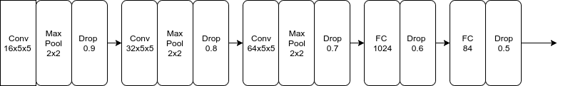
| Layer | Description | |:---------------------:|:---------------------------------------------:| | Input | 32x32x3 RGB image | | Convolution 5x5 | 1x1 stride, same padding, outputs 32x32x16 | | RELU | | | Max pooling | 2x2 stride, outputs 16x16x16 | | DropOut | probability of keeping nodes 0.9 | | Convolution 5x5 | 1x1 stride, same padding, outputs 16x16x32 | | RELU | | | Max Pooling | 2x2 stride, outputs 8x8x32 | | DropOut | probability of keeping nodes 0.8 | | Convolution 5x5 | 1x1 stride, same padding, outputs 8x8x64 | | RELU | | | Max Pooling | 2x2 stride, outputs 4x4x64 | | DropOut | probability of keeping nodes 0.7 | | Fully Connected | Input - 1024 Output - 2048 | | DropOut | probability of keeping nodes 0.6 | | Fully Connected | Input - 2048 Output - 84 | | DropOut | probability of keeping nodes 0.5 | | Fully Connected | Input - 84 Output - 43 |
Testing accuracy of 97.126% Woohoo! But there's one little problem. Can we do away with a fully connected layer ? Let's try that!
| Layer | Description | |:---------------------:|:---------------------------------------------:| | Input | 32x32x3 RGB image | | Convolution 5x5 | 1x1 stride, same padding, outputs 32x32x16 | | RELU | | | Max pooling | 2x2 stride, outputs 16x16x16 | | DropOut | probability of keeping nodes 0.9 | | Convolution 5x5 | 1x1 stride, same padding, outputs 16x16x32 | | RELU | | | Max Pooling | 2x2 stride, outputs 8x8x32 | | DropOut | probability of keeping nodes 0.8 | | Convolution 5x5 | 1x1 stride, same padding, outputs 8x8x64 | | RELU | | | Max Pooling | 2x2 stride, outputs 4x4x64 | | DropOut | probability of keeping nodes 0.7 | | Fully Connected | Input - 1024 Output - 120 | | DropOut | probability of keeping nodes 0.5 | | Fully Connected | Input - 120 Output - 43 |
| Accuracy Type | Accuracy Value | |:---------------------:|:---------------------------------------------:| | Training |93.9 % | | Testing | 96.603% | | Validation | 98.095% |
Hmm. Something wrong there? Let's try modifying the number of nodes in the hiden layer from 120 to 84.
97.625 testing accuracy. Thats more like it.
Activation functions
So far we have used the RELU activation function. How about ELU ? They say the mean value of ELU activation function is zero, leading to faster learning and also, it doesnn't saturate,being an exponential function. Now that we have tried almost everything, let's get this Activation thing sorted with. Hmm.. 96.239% testing accuracy.
Even after restoring the number of fully connected layers to 3, the testing accuracy is still around 96.595
| Accuracy Type | Accuracy Value | |:---------------------:|:---------------------------------------------:| | Training |91.1 % | | Testing | 96.595% | | Validation | 97.868% |
RELU worked better.
Other architectures
Now this is interesting. Since quite a number of myths have been busted, I cannot rule this out. This paper by Yann Lecun presents an interesting method of learning. It suggests providing as input to the fully connected layers, not just the output from the last convolutional layer, but outputs from all the convolutional layers, which would help in propagating the learning from all the convolutional layers to the fully connected layers in a much better way. Lets try this out..
| Accuracy Type | Accuracy Value | |:---------------------:|:---------------------------------------------:| | Testing | 97.158% | | Validation | 97.891% |
Hmm..so near, yet so far.
So I will have to go back to the this previous architecture of 3conv-2fc. And this is our final model.
| Layer | Description | |:---------------------:|:---------------------------------------------:| | Input | 32x32x3 RGB image | | Convolution 5x5 | 1x1 stride, same padding, outputs 32x32x16 | | RELU | | | Max pooling | 2x2 stride, outputs 16x16x16 | | DropOut | probability of keeping nodes 0.9 | | Convolution 5x5 | 1x1 stride, same padding, outputs 16x16x32 | | RELU | | | Max Pooling | 2x2 stride, outputs 8x8x32 | | DropOut | probability of keeping nodes 0.8 | | Convolution 5x5 | 1x1 stride, same padding, outputs 8x8x64 | | RELU | | | Max Pooling | 2x2 stride, outputs 4x4x64 | | DropOut | probability of keeping nodes 0.7 | | Fully Connected | Input - 1024 Output - 84 | | DropOut | probability of keeping nodes 0.5 | | Fully Connected | Input - 120 Output - 43 |
Final results
| Accuracy Type | Accuracy Value | |:---------------------:|:---------------------------------------------:| | Training |93.1 % | | Testing | 97.213% | | Validation | 98.345% |
Test a Model on New Images


Here are the results of the prediction:
| Original Image | Predicted Image | |:---------------------:|:---------------------------------------------:| | Caution | Caution | | 30 speed limit | 30 speed limit | | Turn left Ahead | Turn left Ahead | | Stop | 30 speed limit | | 50 speed limit | 50 speed limit |
The model was able to correctly guess 4 of the 5 traffic signs, which gives an accuracy of 80%.
Image -by Image classification results
Genral caution image
| Probabilities | probability Values | |:---------------------:|:---------------------------------------------:| | Caution | 0.995 | | Traffic Signals | 0.004 | | Pedestrians | 0.0 | | Road narrows on the right | 0.0 | | Road Work | 0.0 |
Thirty speed limit image
| Probabilities | probability Values | |:---------------------:|:---------------------------------------------:| | 30 speed limit | 0.997 | | 50 speed limit | 0.002 | | 80 speed limit | 0.0 | | 70 speed limit | 0.0 | | 20 speed limit | 0.0 |
Turn Left Ahead image
| Probabilities | probability Values | |:---------------------:|:---------------------------------------------:| | Turn left Ahead | 0.99 | | Keep right | 0.00 | | Ahead only | 0.0 | | Stop | 0.0 | | Go striaght or right | 0.0 |
Stop image
| Probabilities | probability Values | |:---------------------:|:---------------------------------------------:| | 30 speed limit | 0.23 | | yield | 0.18 | | Children's crossing | 0.12 | | Bicycles crossing | 0.09 | | Priority Road | 0.08 |
Fifty speed limit image
| Probabilities | probability Values | |:---------------------:|:---------------------------------------------:| | 50 speed limit | 0.99 | | 30 speed limit | 0.01 | | 80 speed limit | 0.00 | | 70 speed limit | 0.0 | | 100 speed limit | 0.0 |
From the softmax probability values, we can see that the model is quite confident (getting about 99% , which is good sign I guess?) about the predictions which it gets right. However the image that it gets wrong (the stop sign image), it doesn't seem quite sure about the predictions with the highest softmax probability ranging around 23% in stark contrast to normal average of 99%.
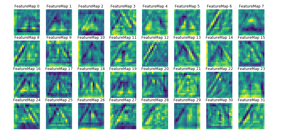
Visualization of feature Maps
Convolution Layer 1 feature maps
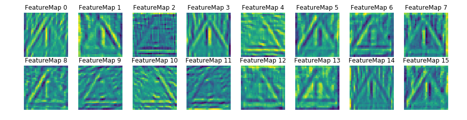
As seen from the visualization, the first convolutional layer picks up the basic shapes such as edges from the image. We can also observe Feature Map 4 getting excited to color Red and feature map 13 to color white.
Convolution Layer 2 feature maps
As seen from the output of the second convolutional layer which seems to picking up from on the output of first layer and trying to recognize blobs (traingle shapes in whole)
Reflections:
This project was quite insightful with regards to how deep learning projects are supposed to be approached. I learnt that it is as much about the network architecture as it is about proper data pre-processing (garbage in, garbage out). The final test accuracy is around 97% which is good, but still not quite there, given people have managed to achieve over 99% accuracy. I'd like to revisit this problem in the future to:
- Try out architectures such as VGG, ResNet and see how they perform compared to current architecture.
- Try out other data balancing approaches.
P.S - Here's the link to the Github Repo.
Piyush Papreja
Software Developer
My research interests include music information retrieval, recommendation systems and web.