Of Monoliths & In-Memory Litter: Building A Music Discovery App - 1
Documenting the lessons from our initial monolithic approach in our discovery system outlined in “Bit Of This, Bit Of That: Revisiting Search & Discovery”
 Photo by Valentino Funghi on Unsplash
Disclaimer 1: This post is the first post in the series about building a music discovery platform based on our paper: Bit Of This, Bit Of That: Revisiting Search and Discovery.
Disclaimer 2: The design choices mentioned in this article are made keeping in mind a low-cost setup. As a result, some of the design choices may not be the most straightforward ones.
Disclaimer 3 You can explore our music discovery platform, This & That Music, here: https://discover.thisandthatmusic.com/.
The term genre-fluid music sounds so fancy and sophisticated and something you aren't supposed to know, yet you do. Even if you didn't realize you did, you do. After all, it's all around us. Think Old Town Road by Lil Nas X. How would you describe its genre? Is it country, or is it hip-hop? Or is it both? And that's what genre fluidity is: any musical item consisting of more than a single genre.
Over the past few decades, genre-fluidity has been gaining prominence in the billboard charts. However, search interfaces have yet to keep up with this trend and continue to be designed for single-genre searches, while genre fluidity is served mostly via recommendations and curated playlists. This may soon change as recent advancements in AI, specifically Large Language Models (LLMs), offer more expansive and expressive access to content.
So why are we talking about genre fluidity and old-town roads? A few years ago, we published a paper proposing a platform to discover genre-fluid music through a combination of expressive search and a user experience created around the core idea of genre-fluid search. This post explains the initial architecture we used to build that discovery system and the lessons we learned.
Search
Our proposed system enables users to search for music by combining different genres and specifying the proportion of each genre they want in the results. We call it genre-fluid search. Adopting the design principles of existing apps, we keep the existing keyword search ("Adele playlists") along with our proposed search to keep the cognitive load as low as possible.
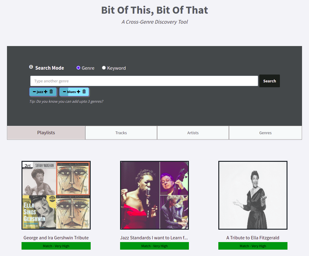
System search modes: Keyword search mode is the conventional search mode, while genre search mode is the proposed one.
Data Summary
Before going into the depth of the architecture, here is a summary of the data used for creating the system:
- There are a total of 88 genres supported by the system.
- There are three entity types: artists, playlists, and tracks.
- The system has around one million playlists, seven million tracks, and a million artists.
- Each entity has demographic data, such as name, popularity, preview audio link, and cover image.
Embeddings
We use neural embeddings for our search and similarity-based recommendation purposes. There are two types of embeddings in our system:
- Genre-based embeddings
- Similarity-based embeddings
To get the genre-based embedding for each entity, we annotate entities with their associated genres so each entity can be represented as an 88-length sparse vector. This vector consists of real values, meaning the nonzero values range between 0 and 1. In addition to entity-genre annotation, we make use of genre relationships and have those relationships reflected in the entity genre annotation.
Similarity-based embeddings are obtained by training word2vec models on our corpus, treating playlists as sentences and tracks (and artists) as words. These embeddings are 300-length vectors, with values ranging between 0 and 1. Finally, to perform Approximate Nearest Neighbor search on our embeddings, we use the Spotify ANNOY library and store the indexes for each entity on disk.
Data Structures And Storage
The main consideration for our search workflow is retrieval as fast as possible, which means it should be memory-based instead of disk or mmap-based. We use the Python pickle module to store our entity details objects as a dictionary, with entity-id being our key and entity details stored in an array ([name, preview audio link, cover image link]). Popularity lookups are stored in the same format as well. We store the sparse genre embeddings as H5 files. Word2vec and Spotify ANNOY data structures are saved as their corresponding supported files.
System Modules
The main components of this system, packaged as a Python Flask application, are:
- Query Parser Module
- Candidate Aggregation Module
- Scoring Module
- Filtering Module
- Detail Population Module
- Caching Module
Query Parser Module
This module converts the search query typed in natural language ("rock with playlists some country") into an 88-genre vector. We apply the genre-relationship rules mentioned in the embeddings section to the query vector.
Candidate Aggregation Module
Even though we create a tree data structure built with binary space partitioning using the Spotify ANNOY library from our genre embeddings, we use our scoring module instead of the conventional query-to-candidate distance as the final scoring metric. We create two indexes per entity type for genre embeddings to get the maximum possible candidates for a given query: one using the Angular distance and another using the Dot Product distance. We sequentially query the indexes and retrieve N=10,000 candidates from the indexes using the candidate aggregator module.
Scoring Module
We use our custom scoring function to calculate a score for each of those 10,000 candidates, where we consider things such as the candidate values corresponding to each query genre, missing genres in a candidate, additional candidate genres not specified in the query, and candidate popularity.
Filtering Module
Since our corpus contains user-created playlists, it is possible to have multiple playlists with the same name. Also, many playlists for a given search query can mainly comprise the same artist. To avoid returning duplicate results in their name or primary artist composition, we have a separate module to filter out such items and finally return K=300 result items sorted by their score.
Detail Population Module
This is where we get details for each result item and prepare the final paginated result set to be sent back to the client.
Caching Module
Since our system serves results without considering user personalization, each query should get the same response. With this in mind, we can cache our query results using Redis, as it is the simplest and the most common solution. We serialize each query as a string and store the indexes returned by the filtering module as the value for each query. Only the query and detail population modules get called for repeated searches, bypassing the rest.
Overall System Design

System Design Architecture `version1`. Monolithic. Simple.
Here's how the application design looks, zoomed out. The query "Rock playlists with blues" is first entered in a search box in a web application.
- The query parser module parses this text and converts it into an 88-length vector.
- The query vector is sent to the server, where the caching module checks whether the query results have already been stored in Redis. In case of a cache hit, steps 3-5 are skipped, and the result set is returned to the browser. In case of a cache miss, the query vector is forwarded to the Candidate Aggregator module.
- The candidate aggregator module uses this query vector to query the Spotify ANNOY indices, retrieves 10000 candidates, and passes it onto the scorer module.
- The scorer module runs our custom scoring function to calculate scores for each of those 10000 candidates.
- The filtering module removes duplicate candidates by name and primary artist. If the resulting set has items under a certain threshold
K, it adds the items removed in the filtering stage. - Finally, the demographic data is retrieved for the first
k=30candidates to be returned to the browser. - Candidates calculated are stored in Redis corresponding to the search query.
- In order to support existing keyword-based searches, we use the PostgreSQL database as it supports full-text search from disk with a decent performance.
Thoughts
The Good
The best thing about this setup is its simplicity. Its monolithic design is as simple as possible, adding little coding complexity overhead. The straightforward nature of this design makes it an ideal choice for prototyping. The design is also modular, making it easier to move away from monolithic architecture in the future. Lastly, using PostgreSQL over other full-text solutions, such as Elasticsearch, works fine without needing the memory most memory-based full-text search solutions need.
The Bad
In-Memory Litter
Using pickle module for serializing data to disk is excellent for entry-level applications and prototypes. They are even more efficient in data storage than other candidates, such as JSON. However, there are better options than pickle when it comes to interoperability, with JSON being one of them. Additionally, moving across different Python versions can also lead to problems.
Another problem that having in-memory objects creates is high memory consumption. While data access is high-speed and straightforward, it also makes deploying the application more complex, as the memory needed for a single instance of the application equals the size of these in-memory objects. This data tied to an instance's memory cannot be shared with other application instances.
Search Time
Owing to our sequential search for Spotify ANNOY indices and the scoring function being run over 10k candidates, the search time is well over 5 seconds for a new query, which is far over the ideal response time.
Caching At A Cost
Caching using Redis is great until it is not. It usually starts with simpler string serialized keys and values, which later becomes a whole thing of writing logic to serialize and deserialize data.
Monolith
The monolithic architecture has notable drawbacks, such as the need to manage, test, and deploy all components as one unit. Additionally, the entire system is bound to a single programming language, which may become less than ideal as the application expands and becomes more complex.
The Ugly
Deploying an application that requires 32GB of memory presents a challenge due to the complexity and high cost of horizontal scaling. For instance, the monthly cost of an AWS t4g.2xlarge instance, which could support such an application, is approximately $180.
Conclusion
The design mentioned above is a decent place to start as it lets the main application idea take focus, owing to its simplicity. Its limiting factors, however, are quite a few and critical as well. Monolith is all well and good up to a certain point, beyond which it stops making sense. In-memory objects lead to substantial memory consumption, complicating the scaling and deployment processes. As we aim to improve this design, our approach would involve reducing memory usage and transitioning from a monolithic structure to a more modular, component-based design.
Until the next design.
Ready to explore genre-fluid music? Visit our music discovery platform, This & Thats Music, here: https://discover.thisandthatmusic.com/
Piyush Papreja
Software Developer
My research interests include music information retrieval, recommendation systems and web.